1.1 - RNN cell
A recurrent neural network can be seen as the repeated use of a single cell. You are first going to implement the computations for a single time-step. The following figure describes the operations for a single time-step of an RNN cell.
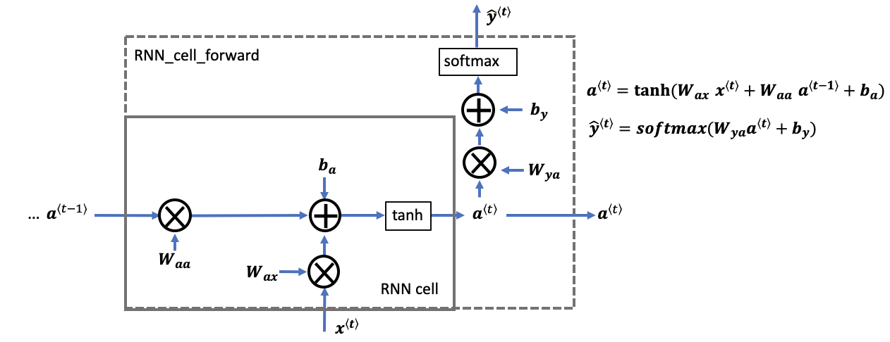
rnn cell versus rnn_cell_forward
- Note that an RNN cell outputs the hidden state \(a^{\langle t \rangle}\).
- The rnn cell is shown in the figure as the inner box which has solid lines.
- The function that we will implement,
rnn_cell_forward, also calculates the prediction \(\hat{y}^{\langle t \rangle}\)- The rnn_cell_forward is shown in the figure as the outer box that has dashed lines.
Implement the RNN-cell described in Figure (2).
Instructions:
1. Compute the hidden state with tanh activation: \(a^{\langle t \rangle} = \tanh(W_{aa} a^{\langle t-1 \rangle} + W_{ax} x^{\langle t \rangle} + b_a)\).
2. Using your new hidden state \(a^{\langle t \rangle}\), compute the prediction \(\hat{y}^{\langle t \rangle} = softmax(W_{ya} a^{\langle t \rangle} + b_y)\). We provided the function softmax.
3. Store \((a^{\langle t \rangle}, a^{\langle t-1 \rangle}, x^{\langle t \rangle}, parameters)\) in a cache.
4. Return \(a^{\langle t \rangle}\) , \(\hat{y}^{\langle t \rangle}\) and cache
def rnn_cell_forward(xt, a_prev, parameters):
    """
    Implements a single forward step of the RNN-cell

    Arguments:
    xt -- your input data at timestep "t", numpy array of shape (n_x, m).
    a_prev -- Hidden state at timestep "t-1", numpy array of shape (n_a, m)
    parameters -- python dictionary containing:
                        Wax -- Weight matrix multiplying the input, numpy array of shape (n_a, n_x)
                        Waa -- Weight matrix multiplying the hidden state, numpy array of shape (n_a, n_a)
                        Wya -- Weight matrix relating the hidden-state to the output, numpy array of shape (n_y, n_a)
                        ba --  Bias, numpy array of shape (n_a, 1)
                        by -- Bias relating the hidden-state to the output, numpy array of shape (n_y, 1)
    Returns:
    a_next -- next hidden state, of shape (n_a, m)
    yt_pred -- prediction at timestep "t", numpy array of shape (n_y, m)
    cache -- tuple of values needed for the backward pass, contains (a_next, a_prev, xt, parameters)
    """

    # Retrieve parameters from "parameters"
    Wax = parameters["Wax"]
    Waa = parameters["Waa"]
    Wya = parameters["Wya"]
    ba = parameters["ba"]
    by = parameters["by"]

    # compute next activation state using the formula given above
    a_next = np.tanh(np.dot(Waa, a_prev) + np.dot(Wax, xt) + ba)
    # compute output of the current cell using the formula given above
    yt_pred = softmax(np.dot(Wya, a_next) + by)

    # store values you need for backward propagation in cache
    cache = (a_next, a_prev, xt, parameters)

    return a_next, yt_pred, cache
np.random.seed(1)
xt_tmp = np.random.randn(3,10)
a_prev_tmp = np.random.randn(5,10)
parameters_tmp = {}
parameters_tmp['Waa'] = np.random.randn(5,5)
parameters_tmp['Wax'] = np.random.randn(5,3)
parameters_tmp['Wya'] = np.random.randn(2,5)
parameters_tmp['ba'] = np.random.randn(5,1)
parameters_tmp['by'] = np.random.randn(2,1)

a_next_tmp, yt_pred_tmp, cache_tmp = rnn_cell_forward(xt_tmp, a_prev_tmp, parameters_tmp)
print("a_next[4] = \n", a_next_tmp[4])
print("a_next.shape = \n", a_next_tmp.shape)
print("yt_pred[1] =\n", yt_pred_tmp[1])
print("yt_pred.shape = \n", yt_pred_tmp.shape)
a_next[4] =
 [ 0.59584544  0.18141802  0.61311866  0.99808218  0.85016201  0.99980978
 -0.18887155  0.99815551  0.6531151   0.82872037]
a_next.shape =
 (5, 10)
yt_pred[1] =
 [0.9888161  0.01682021 0.21140899 0.36817467 0.98988387 0.88945212
 0.36920224 0.9966312  0.9982559  0.17746526]
yt_pred.shape =
 (2, 10)
1.2 - RNN forward pass
- A recurrent neural network (RNN) is a repetition of the RNN cell that you've just built.
- If your input sequence of data is 10 time steps long, then you will re-use the RNN cell 10 times.
- Each cell takes two inputs at each time step:
- \(a^{\langle t-1 \rangle}\): The hidden state from the previous cell.
- \(x^{\langle t \rangle}\): The current time-step's input data.
- It has two outputs at each time step:
- A hidden state (\(a^{\langle t \rangle}\))
- A prediction (\(y^{\langle t \rangle}\))
- The weights and biases \((W_{aa}, b_{a}, W_{ax}, b_{x})\) are re-used each time step.
- They are maintained between calls to rnn_cell_forward in the 'parameters' dictionary.
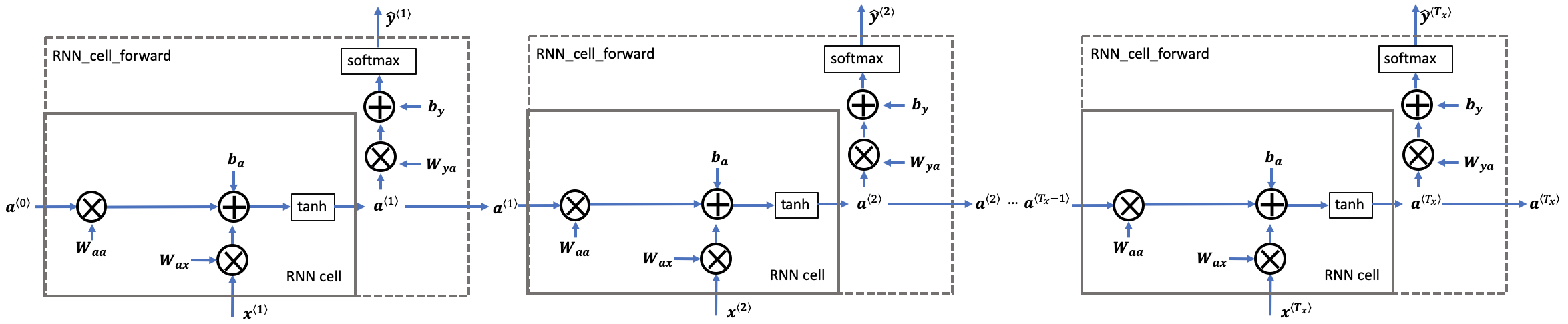
Coding the forward propagation of the RNN described in Figure (3).
Instructions:
Create a 3D array of zeros, \(a\) of shape \((n_{a}, m, T_{x})\) that will store all the hidden states computed by the RNN.
Create a 3D array of zeros, \(\hat{y}\), of shape \((n_{y}, m, T_{x})\) that will store the predictions.
- Note that in this case, \(T_{y} = T_{x}\) (the prediction and input have the same number of time steps).
Initialize the 2D hidden state a_next by setting it equal to the initial hidden state, \(a_{0}\).
At each time step \(t\):
- Get \(x^{\langle t \rangle}\), which is a 2D slice of \(x\) for a single time step \(t\).
- \(x^{\langle t \rangle}\) has shape \((n_{x}, m)\)
- \(x\) has shape \((n_{x}, m, T_{x})\)
- Update the 2D hidden state \(a^{\langle t \rangle}\) (variable name a_next), the prediction \(\hat{y}^{\langle t \rangle}\) and the cache by running rnn_cell_forward.
- \(a^{\langle t \rangle}\) has shape \((n_{a}, m)\)
- Store the 2D hidden state in the 3D tensor \(a\), at the \(t^{th}\) position.
- \(a\) has shape \((n_{a}, m, T_{x})\)
- Store the 2D \(\hat{y}^{\langle t \rangle}\) prediction (variable name yt_pred) in the 3D tensor \(\hat{y}_{pred}\) at the \(t^{th}\) position.
- \(\hat{y}^{\langle t \rangle}\) has shape \((n_{y}, m)\)
- \(\hat{y}\) has shape \((n_{y}, m, T_x)\)
- Append the cache to the list of caches.
* Return the 3D tensor \(a\) and \(\hat{y}\), as well as the list of caches.
def rnn_forward(x, a0, parameters):
    """
    Implement the forward propagation of the recurrent neural network described in Figure (3).

    Arguments:
    x -- Input data for every time-step, of shape (n_x, m, T_x).
    a0 -- Initial hidden state, of shape (n_a, m)
    parameters -- python dictionary containing:
                        Waa -- Weight matrix multiplying the hidden state, numpy array of shape (n_a, n_a)
                        Wax -- Weight matrix multiplying the input, numpy array of shape (n_a, n_x)
                        Wya -- Weight matrix relating the hidden-state to the output, numpy array of shape (n_y, n_a)
                        ba --  Bias numpy array of shape (n_a, 1)
                        by -- Bias relating the hidden-state to the output, numpy array of shape (n_y, 1)

    Returns:
    a -- Hidden states for every time-step, numpy array of shape (n_a, m, T_x)
    y_pred -- Predictions for every time-step, numpy array of shape (n_y, m, T_x)
    caches -- tuple of values needed for the backward pass, contains (list of caches, x)
    """

    # Initialize "caches" which will contain the list of all caches
    caches = []

    # Retrieve dimensions from shapes of x and parameters["Wya"]
    n_x, m, T_x = x.shape
    n_y, n_a = parameters["Wya"].shape

    ### START CODE HERE ###

    # initialize "a" and "y_pred" with zeros (≈2 lines)
    a = np.zeros((n_a, m, T_x))
    y_pred = np.zeros((n_y, m, T_x))

    # Initialize a_next (≈1 line)
    a_next = a0

    # loop over all time-steps of the input 'x' (1 line)
    for t in range(T_x):
        # Update next hidden state, compute the prediction, get the cache (≈2 lines)
        xt = x[:, :, t]
        #print("The shape of xt is :", xt.shape)
        #print("The shape of x is :", x.shape)
        a_next, yt_pred, cache = rnn_cell_forward(xt, a_next, parameters)
        # Save the value of the new "next" hidden state in a (≈1 line)
        #print("The value of a_next is :", a_next)
        a[:,:,t] = a_next
        # Save the value of the prediction in y (≈1 line)
        y_pred[:,:,t] = yt_pred
        # Append "cache" to "caches" (≈1 line)
        caches.append(cache)
    # store values needed for backward propagation in cache
    caches = (caches, x)

    return a, y_pred, caches
np.random.seed(1)
x_tmp = np.random.randn(3,10,4)
a0_tmp = np.random.randn(5,10)

parameters_tmp = {}
parameters_tmp['Waa'] = np.random.randn(5,5)
parameters_tmp['Wax'] = np.random.randn(5,3)
parameters_tmp['Wya'] = np.random.randn(2,5)
parameters_tmp['ba'] = np.random.randn(5,1)
parameters_tmp['by'] = np.random.randn(2,1)

a_tmp, y_pred_tmp, caches_tmp = rnn_forward(x_tmp, a0_tmp, parameters_tmp)
print("a[4][1] = \n", a_tmp[4][1])
print("a.shape = \n", a_tmp.shape)
print("y_pred[1][3] =\n", y_pred_tmp[1][3])
print("y_pred.shape = \n", y_pred_tmp.shape)
print("caches[1][1][3] =\n", caches_tmp[1][1][3])
print("len(caches) = \n", len(caches_tmp))
a[4][1] =
 [-0.99999375  0.77911235 -0.99861469 -0.99833267]
a.shape =
 (5, 10, 4)
y_pred[1][3] =
 [0.79560373 0.86224861 0.11118257 0.81515947]
y_pred.shape =
 (2, 10, 4)
caches[1][1][3] =
 [-1.1425182  -0.34934272 -0.20889423  0.58662319]
len(caches) =
 2
Congratulations! We've successfully built the forward propagation of a recurrent neural network from scratch.
Situations when this RNN will perform better:
- This will work well enough for some applications, but it suffers from the vanishing gradient problems.
- The RNN works best when each output \(\hat{y}^{\langle t \rangle}\) can be estimated using "local" context.
- "Local" context refers to information that is close to the prediction's time step \(t\).
- More formally, local context refers to inputs \(x^{\langle t' \rangle}\) and predictions \(\hat{y}^{\langle t \rangle}\) where \(t'\) is close to \(t\).
In the next part, we will build a more complex LSTM model, which is better at addressing vanishing gradients. The LSTM will be better able to remember a piece of information and keep it saved for many timesteps.