Building your Recurrent Neural Network - Step by Step

We will implement key components of a Recurrent Neural Network in numpy.

Recurrent Neural Networks (RNN) are very effective for Natural Language Processing and other sequence tasks because they have "memory". They can read inputs \(x^{\langle t \rangle}\) (such as words) one at a time, and remember some information/context through the hidden layer activations that get passed from one time-step to the next. This allows a unidirectional RNN to take information from the past to process later inputs. A bidirectional RNN can take context from both the past and the future.

Notation: - Superscript \([l]\) denotes an object associated with the \(l^{th}\) layer.

• Superscript \((i)\) denotes an object associated with the \(i^{th}\) example.

• Superscript \(\langle t \rangle\) denotes an object at the \(t^{th}\) time-step.

• Subscript \(i\) denotes the \(i^{th}\) entry of a vector.

Example:
- \(a^{(2)[3]<4>}_5\) denotes the activation of the 2nd training example (2), 3rd layer [3], 4th time step <4>, and 5th entry in the vector.

Let's first import all the packages that you will need during this assignment.

import numpy as np
from rnn_utils import *

1 - Forward propagation for the basic Recurrent Neural Network

Later this week, you will generate music using an RNN. The basic RNN that you will implement has the structure below. In this example, \(T_x = T_y\).

Dimensions of input \(x\)

Input with \(n_x\) number of units

• For a single timestep of a single input example, \(x^{(i) \langle t \rangle }\) is a one-dimensional input vector.
• Using language as an example, a language with a 5000 word vocabulary could be one-hot encoded into a vector that has 5000 units. So \(x^{(i)\langle t \rangle}\) would have the shape (5000,).
• We'll use the notation \(n_x\) to denote the number of units in a single timestep of a single training example.

Time steps of size \(T_{x}\)

• A recurrent neural network has multiple time steps, which we'll index with \(t\).
• In the lessons, we saw a single training example \(x^{(i)}\) consist of multiple time steps \(T_x\). For example, if there are 10 time steps, \(T_{x} = 10\)

Batches of size \(m\)

• Let's say we have mini-batches, each with 20 training examples.
• To benefit from vectorization, we'll stack 20 columns of \(x^{(i)}\) examples.
• For example, this tensor has the shape (5000,20,10).
• We'll use \(m\) to denote the number of training examples.
• So the shape of a mini-batch is \((n_x,m,T_x)\)

3D Tensor of shape \((n_{x},m,T_{x})\)

• The 3-dimensional tensor \(x\) of shape \((n_x,m,T_x)\) represents the input \(x\) that is fed into the RNN.

Taking a 2D slice for each time step: \(x^{\langle t \rangle}\)

• At each time step, we'll use a mini-batches of training examples (not just a single example).
• So, for each time step \(t\), we'll use a 2D slice of shape \((n_x,m)\).
• We're referring to this 2D slice as \(x^{\langle t \rangle}\). The variable name in the code is xt.

Definition of hidden state \(a\)

• The activation \(a^{\langle t \rangle}\) that is passed to the RNN from one time step to another is called a "hidden state."

Dimensions of hidden state \(a\)

• Similar to the input tensor \(x\), the hidden state for a single training example is a vector of length \(n_{a}\).
• If we include a mini-batch of \(m\) training examples, the shape of a mini-batch is \((n_{a},m)\).
• When we include the time step dimension, the shape of the hidden state is \((n_{a}, m, T_x)\)
• We will loop through the time steps with index \(t\), and work with a 2D slice of the 3D tensor.
• We'll refer to this 2D slice as \(a^{\langle t \rangle}\).
• In the code, the variable names we use are either a_prev or a_next, depending on the function that's being implemented.
• The shape of this 2D slice is \((n_{a}, m)\)

Dimensions of prediction \(\hat{y}\)

• Similar to the inputs and hidden states, \(\hat{y}\) is a 3D tensor of shape \((n_{y}, m, T_{y})\).
  • \(n_{y}\): number of units in the vector representing the prediction.
  • \(m\): number of examples in a mini-batch.
  • \(T_{y}\): number of time steps in the prediction.
• For a single time step \(t\), a 2D slice \(\hat{y}^{\langle t \rangle}\) has shape \((n_{y}, m)\).
• In the code, the variable names are:
  • y_pred: \(\hat{y}\)
  • yt_pred: \(\hat{y}^{\langle t \rangle}\)

Here's how we can implement an RNN:

Steps: 1. Implement the calculations needed for one time-step of the RNN. 2. Implement a loop over \(T_x\) time-steps in order to process all the inputs, one at a time.

1.1 - RNN cell

A recurrent neural network can be seen as the repeated use of a single cell. You are first going to implement the computations for a single time-step. The following figure describes the operations for a single time-step of an RNN cell.

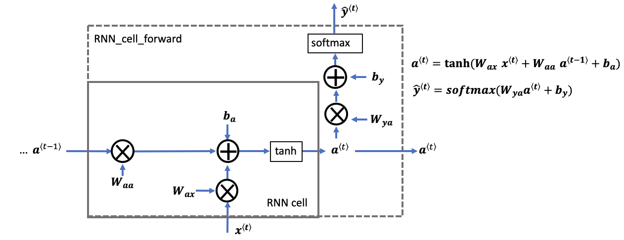
rnn cell versus rnn_cell_forward

• Note that an RNN cell outputs the hidden state \(a^{\langle t \rangle}\).
  • The rnn cell is shown in the figure as the inner box which has solid lines.
• The function that we will implement, rnn_cell_forward, also calculates the prediction \(\hat{y}^{\langle t \rangle}\)
  • The rnn_cell_forward is shown in the figure as the outer box that has dashed lines.